Fun Data for teaching R

I’ll be running an R course soon and I am looking for fun (public) datasets to use in data manipulation and visualization. I would like to use a single dataset that has some easy variables for the first days, but also some more challenging ones for the final days. And I want that when I put exercises, the students* are curious about finding out the answer.

[*in this case students are not ecologists]

Ideas:

-Movies. How many movies has Woody Allen? Is the number of movies per year increasing linearly or exponentially? That is a good theme with lots of options. IMDB releases some data, AND processing their terribly formatted txt files and assembling them would be an excellent exercise for an advanced class, but not for beginners. OMDB has an API to make searches and if you donate you can get the full database. And of course, there is an R package to use the API. This is better option for beginners.

-Music. Everyone likes music and there are 300Gb of data here. You can get also just a chunk, though, but still 2 Gb of data is probably too much for beginers.

-Football: I discarded this one for me because I know nothing about it, but I am sure it will be highly popular in Spain. An open database here.

Kaggel datasets are also awesome. To download them you just have to register. I may use the baby names per year and US state. Everyone is curious about the most popular name the year of your birthday, for example.

Earthquakes: This one also needs some parsing of the txt files (easier than IMDB) and will do for pretty visualizations.

-Datasets already in R: Along with the classic datasets on Iris flowers (used by Fisher!) or the cars dataset there are cooler options. For example there are lots of datasets for econometrics (some are curious), and Rstudio also released some cool ones recently (e.g. flights).

-Other: Internet is full of data like real time series, lots of small data examples, M&M’s colors by bag, Jeopardy questions, Marvel social networks, Dolphins social networks, …

Please, add your ideas in the comments, especially if you have used them with success for teaching R. Thanks!


Power analysis for mixed models

[Update: An updated version of pamm has been submitted to CRAN. See below for his author comments.]

This is a quick note that may be useful for some people. I was interested in knowing how many years of monitoring we need to detect a trend. This is a long term monitoring project, so we already have 7 years of data to play with. For a simple design, you can use the pwr library in R to answer your question, but for nested designs (i.e. random factors) things get hairy. In this and this paper they suggest building your own simulation and both has quite complex supplementary material with R code. I didn’t spent enough time to make sense of them. I also found thanks to @frod_san two packages that do it for you. The first, PAMM,  is broken (lme4 keep evolving, while the package didn’t, so even the example they use don’t work). The second (SimR) is not published yet, but is amazingly simple. All its code is in github and they are fast at fixing any bug you may detect (they fixed a small bug I found in no time). You can find a gist with an example of my question and how I calculate power here: https://gist.github.com/ibartomeus/e8eab8a32b57423341fb


is_invasive( ) got a new best friend: is_native( )

A while ago I did a function to check if a species was among the worst invaders. I am really happy this function was used and ropensci put it in a package. However the function does not tell you if a species is exotic in a particular place, and this is what most people want to know. Scott Chamberlain found a couple of other resources to get invasive species lists and we where discussing where to find those reliable, complete “lists of exotic species per region”, but we where thinking the problem from the wrong approach.

Exotic species lists will be always incomplete and hard to maintain. For most research questions the reverse question is also suited. Instead of “is exotic?”, you can ask “is not native?” Lists of natives species are easier to get and stable through time. Moreover, It conveys the message that any non native species is potentially harmful, rather than restricting to “worst invaders” or “known exotic species”.

So here it is. Its implemented for animals and plants in the US (using ITIS database) and for Plants in Europe (Using Flora Europaea)*. You can use it with the following R code:

install.packages("devtools")
library(devtools)
install_github("ibartomeus/traits")
library("traits")

#make a species list
sp <- c("Lavandula stoechas", "Carpobrotus edulis", "Rhododendron ponticum", "Alkanna lutea", "Anchusa arvensis")

#ask in which countries the first species is native by querying in Flora Europaea
fe_native(sp[1])
?fe_native #to see the help page.

#use sapply for querying all species at once
sapply(sp, fe_native, simplify = FALSE)

#ask if the first species is native in a particular region
is_native(sp[1], where = "Islas_Baleares", region = "europe")
?is_native #to see the help page and country names used

#or all species at once
sapply(sp, is_native, where = "Continental US", region = "america")
sapply(sp, is_native, where = "Islas_Baleares", region = "europe")

#for america I am calling itis_native function from taxize package.

The function will be available from ropensci/traits soon, and probably Scott will make it faster and more usable. Let me know if it breaks with any species or if the help pages needs clarifications and I can try to fix it.

*If you know/have a list of all native species for your region of interest, we can add it.

Getting the most of mix models with random slopes

I use mix models as a way to find general patterns integrating different levels of information (i.e. the random effects). Sometimes you only want to focus on the general effects, but others the variation among levels is also of interest. If this is the case, using a random slope model is pretty cool, but making sense of lmer output is not trivial. I provide here code to get the random slopes and CI’s of such models using the iris dataset in R (mainly, because I am sure I will need to check this entry in the future myself)

#This shows how to get the random slopes and CI's for each level in a hierarchical model

Is there a general relationship between petal and sepal width? and how it differs by species?

plot(iris$Sepal.Width ~ iris$Petal.Width, col = iris$Species, las =1
Uno
#Our model with random slope and intercept
library(lmer)
m2 <- lmer(data = iris, Sepal.Width ~ Petal.Width + (1 + Petal.Width|Species))
#extract fixed effects
a=fixef(m2)
#extract random effects
b=ranef(m2, condVar=TRUE)
# Extract the variances of the random effects
qq <- attr(b[[1]], "postVar")
e=(sqrt(qq)) 
e=e[2,2,] #here we want to access the Petal.Weigth, which is stored in column 2 in b[[1]], that's why I use the [,2,2]
#calculate CI's
liminf=(b[[1]][2]+a[2])-(e*2)
mean_=(b[[1]][2]+a[2])
limsup=(b[[1]][2]+a[2])+(e*2)
#Plot betas and its errors
dotchart(mean_$Petal.Width, labels = rownames(mean_), cex = 0.5,         xlim = c(0.4,1.4), xlab = "betas")
#add CI's...
for (i in 1:nrow(mean_)){
     lines(x = c(liminf[i,1], limsup[i,1]), y = c(i,i)) 
}
dos
#make final plot
plot(iris$Sepal.Width ~ iris$Petal.Width, col = iris$Species, las = 1)
#and plot each random slope
abline(a = b[[1]][1,1]+a[1], b= mean_$Petal.Width[1], col = "black")
abline(a = b[[1]][2,1]+a[1], b= mean_$Petal.Width[2], col = "red")
abline(a = b[[1]][3,1]+a[1], b= mean_$Petal.Width[3], col = "green")
#and general response
abline(a, lty = 2)
tres

The code is fast and dirty, I know I can be more consistent, and the plot can be nicer (clip the slopes, add SE’s), but will work to get the idea.

& thanks to Lucas Garibaldi for sharing much of this knowledge with me.

And the gist: https://gist.github.com/ibartomeus/f493bf142073c704391b

Preferring a preference index

First I like to use a quantitative framework (you can use ranks-based indices as in Williams et al 2011, which has nice properties too). The simplest quantitative index is the forage ratio:

#obs: observed frequency of visits to item 1
#exp: expected frequency of visits to item 1 (i.e. resource abundance/availability)
fr <- function(obs, exp){
    p_obs <- obs/sum(obs)
    p_exp <- exp/sum(exp)
    out <- p_obs/p_exp
    out
}

But it ranges from 0 to infinity, which makes it hard to interpret.

Second, the most used index is “Electivity” (Ivlev 1961), which is nice because is bounded between -1 and 1. “Jacobs” index is similar, but correcting for item depletion, which do not apply to my question, but see below for completness.

electicity <- function(obs, exp){
    p_obs <- obs/sum(obs)
    p_exp <- exp/sum(exp)
    out <- (p_obs-p_exp)/(p_obs+p_exp)
}

jacobs <- function(obs, exp){
    p_obs <- obs/sum(obs)
    p_exp <- exp/sum(exp)
    out <- (p_obs-p_exp)/(p_obs+p_exp-2*p_obs*p_exp)
    out
}

However, those indexes do not tell you if pollinators have general preferences over several items, and which of this items are preferred or not. To solve that we can use a simple chi test. Chi statistics can be used to assess if there is an overall preference. The Chi test Pearson residuals (obs-exp/√exp) estimate the magnitude of preference or avoidance for a given item based on deviation from expected values. Significance can be assessed by building Bonferroni confidence intervals (see Neu et al. 1974 and Beyers and Steinhorst 1984). That way you know which items are preferred or avoided.

chi_pref <- function(obs, exp, alpha = 0.05){
    chi <- chisq.test(obs, p = exp, rescale.p = TRUE)
    print(chi) #tells you if there is an overall preference. (sig = pref)
    res <- chi$residuals
    #res <- (obs-exp)/sqrt(exp) #hand calculation, same result.
    #calculate bonferoni Z-statistic for each plant.
    alpha <- alpha
    k <- length(obs)
    n <- sum(obs)
    p_obs <- obs/n
    ak <- alpha/(2*k)
    Zak <- abs(qnorm(ak))
    low_interval <- p_obs - (Zak*(sqrt(p_obs*(1-p_obs)/n)))
    upper_interval <- p_obs + (Zak*(sqrt(p_obs*(1-p_obs)/n)))
    p_exp <- exp/sum(exp)
    sig <- ifelse(p_exp >= low_interval & p_exp <= upper_interval, "ns", "sig")
    plot(c(0,k+1), c(min(low_interval),max(upper_interval)), type = "n", 
         ylab = "Preference", xlab = "items", las = 1)
    arrows(x0 = c(1:k), y0 = low_interval, x1 = c(1:k), y1 = upper_interval, code = 3
           ,angle = 90)
    points(p_exp, col = "red")
    out <- data.frame(chi_test_p = rep(chi$p.value, length(res)), 
                      chi_residuals = res, sig = sig)
    out
}

And we wrap up all indexes…

#wrap up for all indexes
preference <- function(obs, exp, alpha = 0.05){
    f <- fr(obs, exp)
    e <- electicity(obs, exp)
    #j <- jacobs(obs, exp)
    c <- chi_pref(obs, exp, alpha = alpha)
    out <- data.frame(exp = exp, obs = obs, fr = f, electicity = e, c)
    out
}

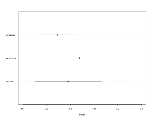
It works well for preferences among items with similar availability, and when all are used to some extent. The plot shows expected values in red, and the observed confidence interval in black. If is not overlapping the expected, indicates a significant preference.

x <- preference(obs = c(25, 22,30,40), exp = c(40,12,12,53))
1
##  Chi-squared test for given probabilities
## 
## data:  obs
## X-squared = 44.15, df = 3, p-value = 1.404e-09
##   exp obs     fr electicity chi_test_p chi_residuals sig
## 1  40  25 0.6250    -0.2308  1.404e-09        -2.372 sig
## 2  12  22 1.8333     0.2941  1.404e-09         2.887  ns
## 3  12  30 2.5000     0.4286  1.404e-09         5.196 sig
## 4  53  40 0.7547    -0.1398  1.404e-09        -1.786 sig

We can see that indices are correlated by simulating lots of random values.

x <- preference(obs = sample(c(0:100),100), exp = sample(c(0:100),100))
##  Chi-squared test for given probabilities
## 
## data:  obs
## X-squared = Inf, df = 99, p-value < 2.2e-16
pairs(x[,c(-5,-7)]) #more or less same patern, across indexes.

2

But the indexes do not behave well in two situations. First, when an item is not used, it is significanly un-preferred regardless of its abundance. I don’t like that, because a very rare plant is expected to get 0 visits from a biological point of view. This is an issue when building bonferroni intervals around 0, which are by definition 0, and any value different from 0 appears as significant.

x <- preference(obs = c(0,25,200), exp = c(0.00003,50,100))
3
##  Chi-squared test for given probabilities
## 
## data:  obs
## X-squared = 50, df = 2, p-value = 1.389e-11
##     exp obs     fr electicity chi_test_p chi_residuals sig
## 1 3e-05   0 0.0000    -1.0000  1.389e-11     -0.006708 sig
## 2 5e+01  25 0.3333    -0.5000  1.389e-11     -5.773502 sig
## 3 1e+02 200 1.3333     0.1429  1.389e-11      4.082486 sig

The second issue is that if you have noise due to sampling (as always), rare items are more likely to be wrongly assessed than common items.

#assume no preferences
x <- preference(obs = c(5,50,100), exp = c(5,50,100))
4
##  Chi-squared test for given probabilities
## 
## data:  obs
## X-squared = 0, df = 2, p-value = 1
##   exp obs fr electicity chi_test_p chi_residuals sig
## 1   5   5  1          0          1             0  ns
## 2  50  50  1          0          1             0  ns
## 3 100 100  1          0          1             0  ns
#now assume some sampling error of +-4 observations
x <- preference(obs = c(1,54,96), exp = c(5,50,100))
5
##  Chi-squared test for given probabilities
## 
## data:  obs
## X-squared = 3.671, df = 2, p-value = 0.1595
##   exp obs     fr electicity chi_test_p chi_residuals sig
## 1   5   1 0.2053  -0.659341     0.1595       -1.7539 sig
## 2  50  54 1.1086   0.051508     0.1595        0.7580  ns
## 3 100  96 0.9854  -0.007338     0.1595       -0.1438  ns

As a conclusion, If you have all items represented (not highly uneven distributions) or all used to some extent (not 0 visits) this is a great tool.

Happy to know better options in the comments, if available.

Gist with the code of this post here.

How to update and backup a MySQL database under version control and all within Rstudio

I am trying to have better workflows to ensure data quality and two important things for me are first, scripting as much as posible the data manipulation process, and second, backing up the database we use under version control (e.g. Git*). I succeeded on that, but it was a 11 TAB problem**, so I though would be good post it here for others, and for my future self.

One goal of the task is to be able to do everything within the same program (Rstudio) for simplicity, so the task implies connecting R to MySQL server via RMySQL, update the database, make a backup copy from R and commit changes.

1) Running mysqldump from R to make an initial backup: RMySQL can’t (that I know) run the most commonly used backup mysqldump. But you can do it by calling the shell (aka Terminal) from R with the function system{base}.

#first we can see which is our path on the shell/terminal
system("pwd") #it should be the working directory.
#Second, we make a mysqldump (has to be in one non broken line,
 #sorry beautiful 80 characters-max code lines)
system("/Applications/MAMP/Library/bin/mysqldump -u USER -h HOSP_IP -pPASWORD --port=8889 --skip-extended-insert DATABASE > DATABASE.sql")
#note that my mysqldump is located in applications folder because 
 #instaled MySQL using MAMP (highly recommended for an easy set up 
 #of a local MySQL environment in a Mac). 
 #Yours may be in /usr/local/mysq/bin/mysqldump
#The --skip-extended-insert makes a INSERT for each row, 
 #which makes version control lighter and more readable later on.

2) Put the backup under version control. Rstudio provide a nice hook to git, so you just need to ‘git init‘ the directory, ‘git add DATABASE.sql‘  and ‘git commit‘ the changes with a nice commit message.

3) Connecting R to MYSQL server to update it: There are good tutorials on this, so I’ll be brief. In this example I manipulated data within R (your.data.frame) and want to append the resulting dataframe to an existing table.

library(RMySQL)
source(psw.R) # this is a way to avoid committing your password. 
 #You can have an r file (added to .gitignore) with the line 
 #psw <- "mypassword", which you can call later from the code.
conn <- dbConnect(dbDriver("MySQL"), user = "USER", 
                  password = psw, dbname="DATABASE", 
                  port = 8889 , host= "HOST_IP") 
#this set up the connection.
dbListTables(conn) # show tables
dbWriteTable(conn, "TABLE", your.data.frame, append = TRUE, 
             overwrite=FALSE, row.name=FALSE) 
#adds the new rows at the bottom of the table.
dbDisconnect(conn) #always disconnect at the end.

4) Make another backup:

system("/Applications/MAMP/Library/bin/mysqldump -u USER -h HOSP_IP -pPASWORD --port=8889 --skip-extended-insert DATABASE > DATABASE.sql")

5) And finally you can make another commit reflecting the changes ‘git add DATABASE.sql‘  and ‘git commit’ with a nice commit message. You can compare the two versions now, and let anyone in the project play with it by pushing it to a central repo (e.g. Github).

I am sure there are other ways to do this, but I am pretty happy of how it works!

—-
*Git forces you to not only document changes, but explain why those changes are done in a nice story. So I prefer it to Audit Trail options in MySQL.
**Someone on the internet suggested to rate the difficulty of a problem in  the number of browser tabs you need to open in order to fix it. Sorry I forgot the source.

On Functional Diversity metrics

Summary: FD is getting very popular, so I figured that would be good to post not only the code (mostly borrowed) I am using: https://github.com/ibartomeus/fundiv, but also what I learnt of it. This posts assume you have read about FD calculation a bit.

I’ve been working with functional diversity (FD) for a couple of years now, and some papers are to come applying this concept to pollinator (and other insect). You can find some help on calculation FD in Owen Petchey‘s webpage and in FD package. However,  Petchey’s et al FD is not in an easy to use R function, so I uploaded some wrap up R functions to calculate the principal indexes, along with some null models and other stuff. There is a brief explanation on how to install and use the package there. But first some background: FD calculates the diversity of traits present in the community, and is a cool concept, because at a same number of species, a community can have quite homogenous or diverse traits, and this can be important to depict mechanisms of ecosystem functioning or responses to global change. However I have a hate-love relationship with the concept.

The first obvious one is that which traits are considered will directly affect the conclusions you get. The garbage in -> garbage out concept applies here, but even if you try to select appropriate traits, trait information quality is usually not good for most species, we don’t know what traits are responsible for which functions and any choice of traits is more subjective than a simple tally of species richness (or Phylogenetic diversity). However, if you identify traits that are meaningful for your question (e.g. body size is the usual suspect), can potentially be a very powerful tool.

A second big problem is that there is quite a few metrics out there. Just reading the literature is quite daunting, so I`ll give you my opinion after implementing them in R and using them on a lot of different datasets. First problem is that Functional diversity calculated as a dendrogram (Petchey approach) or as a space based (FD package approach) metric is not equivalent (they are correlated, but not strongly), and this is bothering me. If I have to choose, I like better dendogram based solutions. Why? You have the ability to calculate FD for communities with very few species (even richness = 1 species). This is useful sometimes, especially with simulations of random species removal. You can easily visualize the dendogram, but not a 8D space. For me dendograms are also easier to understand than PCoA’s. Moreover, the original distance matrix used tend to be better described by dendograms than by PCoA’s (in several datasets). Space based calculations crash more often than one would want and you are forced to drop lots of axes to calculate hypervolums (and sometimes is impossible to get some metrics for concrete datasets). Also, Feve and Fdiv are hard to interpret for me, even after reading about them several times. Said so, I have to say that we found Feve to predict fairly good function, and better than dendogram based indexes. Dendrogram based indexes are not perfect either, and specially they need for a better coverage of different complementary metrics, including not only Frich, but also equivalents of Feve and Fdis. I developed a weighted version of Frich (see link to package above), and an evenness one can be easily calculated using phylogenetic imbalance metrics (or see treeNODF!). If anyone is interested in exploring this options further drop me an email.

About Data

I recently did a workshop about data with PhD students. That was great to order my thoughts and put together a lot of good resources. All material used (with lots of links) is available in GitHub: https://github.com/ibartomeus/Data. Topics range from hardcore R code to read, clean and transform data, to discussions about data sharing and reproducibility. Few PhD students thought about sharing their data before the workshop, and I hope I convinced some of them, not sure about that. However, I clearly convinced them to have reproducible workflows and ditch excel, which is a win.

In the last years I worked with lots of different data (mine and from others, big and small) and I have to say most datasets were poorly formated, maintained and documented. I think we do not give enough importance to data curating practices, but they are central to the scientific process. The feedback of the students is that the workshop was very enlightening for them and that they never received formal or informal advice on how to deal with data. If things are going to change, we need to do an active effort to form the new generation of scientists in a open data culture.

Quick and dirty notes on General Linear Mix Models

My datasets tend to have random factors. I try to stick to general models whenever I can to avoid dealing with both random factors and complex error distributions (not always possible). I am compiling some notes here to avoid visiting the same R-forums every time I work in a new project. Those are some notes to self, but may be they are useful to someone else. Note that those are oversimplified notes, they assume you know your stats and your R and only want a cheat sheet. Also, they may contain errors/discrepancies with your philosophy (please notify me if you find errors, so I can update it!)

Only piece of advice. Plot everything and understand your data.

I’ll designate:
Response variable –this is what we want to model as y.
Predictors –This is what we think is affecting the response variable as xz when continuos, and AB when discrete with levels denoted by A1A2, etc… 

Models abbreviated as m.

Let’s start assuming normal error distributions:

1) Easy linear model with one predictor:

    m <- lm(y ~ x)

then check residuals. You want to see no pattern in the following plot:

    scatter.smooth(residuals(m)~fitted(m))

and a straight line here 

    qqPlot(residuals(m))

    qqline(residuals(m))

more diagnostics here: http://www.statmethods.net/stats/rdiagnostics.html

2) Let’s say you have also a Covariate z

    m <- lm(y ~ z + x)

    summary(m)

    coef(m)

    confint(m)

If you want the anova table

    anova(m)

But the covariable should be added first because order matters. The result will be the variance explained by x after accounting for the variance due to A (that’s call a Type 1 error)

3) Otherwise what you actually have is not a covariable, but two predictors:

    m <- lm(y ~ z + x)

    summary(m) #same here

    library(car)

    Anova(m, Type = "II")

If there is indeed no interaction, then type II is statistically more powerful than type III

If the interaction is significant type III is more appropriate

    m <- lm(y ~ z * x)

    summary(m)

    library(car)

    Anova(m, Type = "III")

note: when your design is classic balanced ANOVA design, it doesn’t matter as all types gives you the same answer. More info here: http://mcfromnz.wordpress.com/2011/03/02/anova-type-iiiiii-ss-explained/

To plot interactions:

    interaction.plot(A, B, y)
    #only works with A and B factors, so it rarely works for me

Or customize it by discretizing one of the variables (e.g. cut(z)) and fit lines for the two/three levels of z using the coefficients.

UPDATE: use predict for this

newdata <- data
newdata$z <- 0 #chose a representative low value to fix
model_pred_lowz <- predict(m, newdata, level = 0) #use level 0 to see         the population level (i.e. not interested in random factors)
plot(y ~ x)
lines(x, model_pred_lowz)
newdata$z <- 1 #chose a high value now
model_pred_highz <- predict(m, newdata, level = 0)
lines(x, model_pred_highz)

Also, if you have NA values, use na.exclude, not na.omit in the model, to add NA’s to the residuals.

4) How? By understanding the output, tricky specially when covariate is a factor.

    m <- lm(y ~ A * x)

    summary(m)

  • (Intercept) Value is the intercept for A1 (v1)
  • A2 value (v2) is the difference in the intercept between A1 and A2 (the intercept for A2 is calculated as v1-v2)
  • x Value is the slope for x given A1 (v3)
  • x:A2 Value (v4) is the difference in the slope for x between A1 and A2 (the slope of x for A2 is calculated as v3-v4)

5) Select models (by AIC or compare two models anova I know confusing name)

    AIC(m)

    library(MuMIn)

    AICc(m) #for small sample size

    anova(m1,m2)

But see below with random factors

6) Until now we wanted to see if there were differences among levels of A.

A included as fixed factor -> “the expectation of the distribution of effects”

    lm(x ~ A + z)

But if we want to see if there are general trends regardless of A, but we want to control for the variability due to A. –> “average effect in the population”, we use:

a) random intercept model (we expect the trend to be equal, but some plants will differ on the intercept)

    library(nlme)

    lme(y ~ x, random = ~1 | A)

b) random slope model (we expect the trend to be dependent on species identity)

    lme(y ~ x, random = ~1 + x | A)

In addition, now we can extract the random effects

    m$coefficients

fixed and random factors, so we can see the random intercepts (and slopes) as well as

    intervals(m)

7) To compare models in nlme

With different radom structures you should use method="REML" as an option. To compare models with different fix effects structure using anova use ML, but give final p-values with REML

8) With complex models you can drege them to find the best ones

    library(MuMIn)

    m_set = dredge(m_full)

    (top_m = get.models(m_set, subset = delta<3))

and compute averages the regular way without shrinkage:

     model.avg(top_m)$avg.model

See also names and str(model.avg(top_m))

Or estimates with shrinkage (zero method) – this makes the most difference for the less important predictors since they will get averaged with a bunch of zeros, probably: model.avg(top_m)$coef.shrinkage

9) But what if residuals are bad?

Don’t panic yet. Some times is because variance is different across groups/values, you can investigate that by:

    boxplot(A, residuals(m, type = "norm"))

    plot(A, residuals(m, type = "norm"))

and fix it by incuding a variance factor in the models weights=varIdent(form=~1|A) (for factors) or weights= varPower(form=~x) for continous variables (you can also try VarExp or varConstPower)

And to check if it worked:

    plot(residuals(m, type = "normalized") ~ fitted(m))

The ref is Cleasby IR, Nakagawa S. 2011. Neglected biological patterns in the residuals. Behavioral Ecology and Sociobiology, 65(12), 2361-2372.

note that lm can not use the weights option, but I think, but you can use gls, instead.

10) Is also recomended to center scale(x, scale = FALSE) or scale scale(x) predictors.

Reference: Schielzeth, H. (2010), Simple means to improve the interpretability of regression coefficients. Methods in Ecology and Evolution, 1: 103–113.

11) You should also worry about co-linearity

    library(car)

    vif(m)

Should be lower than 2.5, and you should be very concerned when is over 10

or for lme’s load this little function from here (https://github.com/aufrank/R-hacks/blob/master/mer-utils.R)

    vif.mer <- function (fit) {
                  ## adapted from rms::vif
v <- vcov(fit)
nam <- names(fixef(fit))
## exclude intercepts
ns <- sum(1 * (nam == "Intercept" | nam == " (Intercept)"))
if (ns > 0) {
v <- v[-(1:ns), -(1:ns), drop = FALSE]
nam <- nam[-(1:ns)] }
d <- diag(v)^0.5
v <- diag(solve(v/(d %o% d)))
names(v) <- nam
                                    v }

    vif.mer(m)

12) and you may want to get R2 for glm also…

Based in Nakagawa, S., Schielzeth, H. (2013), A general and simple method for obtaining R2 from generalized linear mixed-effects models. Methods in Ecology and Evolution, 4: 133–142.

    library(MuMIn)

    r.squaredGLMM(m)

——————————————————————————————————

More details and plotting here: https://www.zoology.ubc.ca/~schluter/R/fit-model/

For GLMM’s (generalized) there is a whole new set of tricky things, maybe will be another gist.

Science at the speed of light

May be is not going that fast, but at the speed of R at least. And R is pretty quick. This has pros and cons. I think that understanding the drawbacks is key to maximize the good things of speed, so here are a few examples.

I have a really awful excel file with a dozen sheets calculating simple diversity indexes and network parameters from my dissertation. I also paste in there the output of Atmar and Patterson Nested Calculator (an .exe program!) and of the MATLAB code that Jordi Bascompte kindly send me to run his nestedness null model. I also used Pajek to plot the networks and calculate some extra indices. It took me at least a year to perform all those calculations and believe me, it will take me another year to be able to reproduce those steps again. That was only 6 years ago. Now, I can have nicer plots and calculate way more indexes than I want in less than 5 minutes using the bipartite package, and yes, is fully reproducible. On the other hand I really understood what I was doing, while running bipartite is completely black-boxy for most people.

Last year I also needed a plant phylogeny to test phylogenetic diversity among different communities. I was quite impressed to find the very useful Phylomatic webpage. I only had to prepare the data in the right format and get the tree. Importing the tree to R proved challenging for a newcomer and I had to tweak the tree in Mesquite beforehand. So yes, time-consuming and not reproducible, but I thought it was extremely fast and cool way to get phylogenies. Just one year after that, I can do all that from my R console thanks to the ropensci people (package taxize). Again, faster, easier, but I also need less knowledge on how that phylogeny is built. I am attaching the simple workflow I used below, as it may be useful. Thanks to Scott Chamberlain for advice on how to catch the errors on the retrieved family names.

library(taxize)
#vector with my species
spec <- c("Poa annua", "Abies procera", "Helianthus annuus")

#prepare the data in the right format (including retrieving family name)
names <- lapply(spec, itis_phymat_format, format='isubmit')

#I still have to do manually the ones with errors
names[grep("^na/", names, value = FALSE, perl = TRUE)]
#names[x] <- "family/genus/genus_species/" #enter those manually

#get and plot the tree
tree <- phylomatic_tree(taxa = names, get = "POST", taxnames=FALSE, parallel=FALSE)
tree$tip.label <- capwords(tree$tip.label)
plot(tree, cex = 0.5)

Finally, someone told me he found an old professor’s lab notebook with schedules of daily tasks (sorry I am terrible with details). The time slot booked to perform an ANOVA by hand was a full day! In this case, you really have to think very carefully which analysis you want to do beforehand. Nowadays speed is not an issue to perform most analysis (but our students will still laugh at our slow R code in 5 years!). Speed can help advance science, but with a great power comes great responsibility. Hence, now is more necessary than ever to understand what we do, and why we do it. I highly recommend to read about recent discussions on the use of sensible default values or the problem of increasing researcher degrees of freedom if you are interested in that topic.