On Functional Diversity metrics

Summary: FD is getting very popular, so I figured that would be good to post not only the code (mostly borrowed) I am using: https://github.com/ibartomeus/fundiv, but also what I learnt of it. This posts assume you have read about FD calculation a bit.

I’ve been working with functional diversity (FD) for a couple of years now, and some papers are to come applying this concept to pollinator (and other insect). You can find some help on calculation FD in Owen Petchey‘s webpage and in FD package. However,  Petchey’s et al FD is not in an easy to use R function, so I uploaded some wrap up R functions to calculate the principal indexes, along with some null models and other stuff. There is a brief explanation on how to install and use the package there. But first some background: FD calculates the diversity of traits present in the community, and is a cool concept, because at a same number of species, a community can have quite homogenous or diverse traits, and this can be important to depict mechanisms of ecosystem functioning or responses to global change. However I have a hate-love relationship with the concept.

The first obvious one is that which traits are considered will directly affect the conclusions you get. The garbage in -> garbage out concept applies here, but even if you try to select appropriate traits, trait information quality is usually not good for most species, we don’t know what traits are responsible for which functions and any choice of traits is more subjective than a simple tally of species richness (or Phylogenetic diversity). However, if you identify traits that are meaningful for your question (e.g. body size is the usual suspect), can potentially be a very powerful tool.

A second big problem is that there is quite a few metrics out there. Just reading the literature is quite daunting, so I`ll give you my opinion after implementing them in R and using them on a lot of different datasets. First problem is that Functional diversity calculated as a dendrogram (Petchey approach) or as a space based (FD package approach) metric is not equivalent (they are correlated, but not strongly), and this is bothering me. If I have to choose, I like better dendogram based solutions. Why? You have the ability to calculate FD for communities with very few species (even richness = 1 species). This is useful sometimes, especially with simulations of random species removal. You can easily visualize the dendogram, but not a 8D space. For me dendograms are also easier to understand than PCoA’s. Moreover, the original distance matrix used tend to be better described by dendograms than by PCoA’s (in several datasets). Space based calculations crash more often than one would want and you are forced to drop lots of axes to calculate hypervolums (and sometimes is impossible to get some metrics for concrete datasets). Also, Feve and Fdiv are hard to interpret for me, even after reading about them several times. Said so, I have to say that we found Feve to predict fairly good function, and better than dendogram based indexes. Dendrogram based indexes are not perfect either, and specially they need for a better coverage of different complementary metrics, including not only Frich, but also equivalents of Feve and Fdis. I developed a weighted version of Frich (see link to package above), and an evenness one can be easily calculated using phylogenetic imbalance metrics (or see treeNODF!). If anyone is interested in exploring this options further drop me an email.

About Data

I recently did a workshop about data with PhD students. That was great to order my thoughts and put together a lot of good resources. All material used (with lots of links) is available in GitHub: https://github.com/ibartomeus/Data. Topics range from hardcore R code to read, clean and transform data, to discussions about data sharing and reproducibility. Few PhD students thought about sharing their data before the workshop, and I hope I convinced some of them, not sure about that. However, I clearly convinced them to have reproducible workflows and ditch excel, which is a win.

In the last years I worked with lots of different data (mine and from others, big and small) and I have to say most datasets were poorly formated, maintained and documented. I think we do not give enough importance to data curating practices, but they are central to the scientific process. The feedback of the students is that the workshop was very enlightening for them and that they never received formal or informal advice on how to deal with data. If things are going to change, we need to do an active effort to form the new generation of scientists in a open data culture.

Short guideline on multi-authored papers.

After being on the two sides of the story (first author and one more of dozens of co-authors) I already made a few errors someone may find useful to know, specially since multi-author papers (more than 10-15 authors from different institutes) are becoming normal (and I am not judging if this is good or bad*, is just happening).

1. Talk about co-authorship early on, but with conditions. This things should be talked at the beginning of the collaboration, because there is nothing more awkward than someone thinking that he/she is coauthoring a paper, while the lead author thinks that he/she is a data provider. However, do not grant co-authorship before even starting the project. Make clear that someone will be a co-author if his/her contribution is [fill in here your expectations] (e.g. the data provided ends up being critical for the paper, you are engaged on ms writing, etc…). By clear I meant very clear.

2. Establish feed-back points. This one is very tricky, because first authors (or the core team leading the paper) do not want 50 people commenting in every decision, but they don’t want coauthors to end up not contributing much. On the other hand, some coauthors want to be more involved than others, but they need to be offered the opportunity to contribute in order to do so. I would recommend to fix at least three points to provide feed-back. First a draft of the questions, hypothesis to be tested and which approach will be used. Second a draft with the main results/ figures. And third a first draft of the paper. Even this seems really a minimum, I made myself the error of not sending almost anything before the complete draft of the paper was ready to some coauthors.

3. Make all correspondence open. Always include all coauthors in the emails with drafts or results to discuss. All coauthors should be able to see other people comments. This is specially important when two coauthors disagree on something. The lead author has the final word, but other coauthors should discuss the disagreement between them (and hopefully agree on something) and in front of all other coauthors.

4. Be clear on what you want. That applies also to both sides. As a first author is very useful to tell people what do you want from them. Instead of letting people comment on whatever they want (they will do that anyway), ask for specific questions. Can some native speaker check my grammar? Can you go trough the mathy part and make sure it is correct? With several coauthors you have the risk that everyone will hope the other will look on the three pages of equations, and no-one ends up doing it. As a co-author is always nice also to state on what do you want to contribute. Even if you think that you will be “near the end of the list”, if you want to be more engaged and have clear ideas on how to redo an analysis, or enhance a figure, say it! (Author order is /should be flexible, so you may end up among firsts authors if you contribute)

Lastly, those are just suggestions, and all of them refer to one basic idea: enhance communication.

*I do think more than 10 authors are rarely useful…

Pollinator contribution to yield quality (and my preprint experience)

I already shared a preprint and post about this paper some time ago, but now is officially peer reviewed and online. You can download the final version here: https://peerj.com/articles/328/

My experience with preprints? The publication process at ThePeerJ was super fast (~ 3 months from submission to publication). In this 3 months 84 people visited the PrePrint and only 52 downloaded the PDF. Nobody commented on it. Taking into account that we are 11 authors (who should account for some of this downloads), you may think that the visibility of the paper didn’t increase much from being out there in advance, but I can prove you wrong. Maybe not much people read it, but I was contacted by one PhD student with a question about the paper. She was working on the topic and preparing the next filed season, so for her, reading it in January, instead of in April was useful. Plus, she found it by google-ing about the topic, proving that preprints are discoverable. So, not always by publishing preprints you reach more people, or get amazing feedback, but at least you can reach the right people, and that’s important enough for me.

I have a guest post in Practical Management blog

Quick note to say I am very glad to have a guest post in an awesome blog about data management, a neglected topic that affect all scientists. The blog is quite funny also, bringing some glamour to the art of data processing. Thanks Christie for inviting me to contribute!

The post is about style, check it out here: http://practicaldatamanagement.wordpress.com/2014/02/24/guest-post-about-style/

Quick and dirty notes on General Linear Mix Models

My datasets tend to have random factors. I try to stick to general models whenever I can to avoid dealing with both random factors and complex error distributions (not always possible). I am compiling some notes here to avoid visiting the same R-forums every time I work in a new project. Those are some notes to self, but may be they are useful to someone else. Note that those are oversimplified notes, they assume you know your stats and your R and only want a cheat sheet. Also, they may contain errors/discrepancies with your philosophy (please notify me if you find errors, so I can update it!)

Only piece of advice. Plot everything and understand your data.

I’ll designate:
Response variable –this is what we want to model as y.
Predictors –This is what we think is affecting the response variable as xz when continuos, and AB when discrete with levels denoted by A1A2, etc… 

Models abbreviated as m.

Let’s start assuming normal error distributions:

1) Easy linear model with one predictor:

    m <- lm(y ~ x)

then check residuals. You want to see no pattern in the following plot:

    scatter.smooth(residuals(m)~fitted(m))

and a straight line here 

    qqPlot(residuals(m))

    qqline(residuals(m))

more diagnostics here: http://www.statmethods.net/stats/rdiagnostics.html

2) Let’s say you have also a Covariate z

    m <- lm(y ~ z + x)

    summary(m)

    coef(m)

    confint(m)

If you want the anova table

    anova(m)

But the covariable should be added first because order matters. The result will be the variance explained by x after accounting for the variance due to A (that’s call a Type 1 error)

3) Otherwise what you actually have is not a covariable, but two predictors:

    m <- lm(y ~ z + x)

    summary(m) #same here

    library(car)

    Anova(m, Type = "II")

If there is indeed no interaction, then type II is statistically more powerful than type III

If the interaction is significant type III is more appropriate

    m <- lm(y ~ z * x)

    summary(m)

    library(car)

    Anova(m, Type = "III")

note: when your design is classic balanced ANOVA design, it doesn’t matter as all types gives you the same answer. More info here: http://mcfromnz.wordpress.com/2011/03/02/anova-type-iiiiii-ss-explained/

To plot interactions:

    interaction.plot(A, B, y)
    #only works with A and B factors, so it rarely works for me

Or customize it by discretizing one of the variables (e.g. cut(z)) and fit lines for the two/three levels of z using the coefficients.

UPDATE: use predict for this

newdata <- data
newdata$z <- 0 #chose a representative low value to fix
model_pred_lowz <- predict(m, newdata, level = 0) #use level 0 to see         the population level (i.e. not interested in random factors)
plot(y ~ x)
lines(x, model_pred_lowz)
newdata$z <- 1 #chose a high value now
model_pred_highz <- predict(m, newdata, level = 0)
lines(x, model_pred_highz)

Also, if you have NA values, use na.exclude, not na.omit in the model, to add NA’s to the residuals.

4) How? By understanding the output, tricky specially when covariate is a factor.

    m <- lm(y ~ A * x)

    summary(m)

  • (Intercept) Value is the intercept for A1 (v1)
  • A2 value (v2) is the difference in the intercept between A1 and A2 (the intercept for A2 is calculated as v1-v2)
  • x Value is the slope for x given A1 (v3)
  • x:A2 Value (v4) is the difference in the slope for x between A1 and A2 (the slope of x for A2 is calculated as v3-v4)

5) Select models (by AIC or compare two models anova I know confusing name)

    AIC(m)

    library(MuMIn)

    AICc(m) #for small sample size

    anova(m1,m2)

But see below with random factors

6) Until now we wanted to see if there were differences among levels of A.

A included as fixed factor -> “the expectation of the distribution of effects”

    lm(x ~ A + z)

But if we want to see if there are general trends regardless of A, but we want to control for the variability due to A. –> “average effect in the population”, we use:

a) random intercept model (we expect the trend to be equal, but some plants will differ on the intercept)

    library(nlme)

    lme(y ~ x, random = ~1 | A)

b) random slope model (we expect the trend to be dependent on species identity)

    lme(y ~ x, random = ~1 + x | A)

In addition, now we can extract the random effects

    m$coefficients

fixed and random factors, so we can see the random intercepts (and slopes) as well as

    intervals(m)

7) To compare models in nlme

With different radom structures you should use method="REML" as an option. To compare models with different fix effects structure using anova use ML, but give final p-values with REML

8) With complex models you can drege them to find the best ones

    library(MuMIn)

    m_set = dredge(m_full)

    (top_m = get.models(m_set, subset = delta<3))

and compute averages the regular way without shrinkage:

     model.avg(top_m)$avg.model

See also names and str(model.avg(top_m))

Or estimates with shrinkage (zero method) – this makes the most difference for the less important predictors since they will get averaged with a bunch of zeros, probably: model.avg(top_m)$coef.shrinkage

9) But what if residuals are bad?

Don’t panic yet. Some times is because variance is different across groups/values, you can investigate that by:

    boxplot(A, residuals(m, type = "norm"))

    plot(A, residuals(m, type = "norm"))

and fix it by incuding a variance factor in the models weights=varIdent(form=~1|A) (for factors) or weights= varPower(form=~x) for continous variables (you can also try VarExp or varConstPower)

And to check if it worked:

    plot(residuals(m, type = "normalized") ~ fitted(m))

The ref is Cleasby IR, Nakagawa S. 2011. Neglected biological patterns in the residuals. Behavioral Ecology and Sociobiology, 65(12), 2361-2372.

note that lm can not use the weights option, but I think, but you can use gls, instead.

10) Is also recomended to center scale(x, scale = FALSE) or scale scale(x) predictors.

Reference: Schielzeth, H. (2010), Simple means to improve the interpretability of regression coefficients. Methods in Ecology and Evolution, 1: 103–113.

11) You should also worry about co-linearity

    library(car)

    vif(m)

Should be lower than 2.5, and you should be very concerned when is over 10

or for lme’s load this little function from here (https://github.com/aufrank/R-hacks/blob/master/mer-utils.R)

    vif.mer <- function (fit) {
                  ## adapted from rms::vif
v <- vcov(fit)
nam <- names(fixef(fit))
## exclude intercepts
ns <- sum(1 * (nam == "Intercept" | nam == " (Intercept)"))
if (ns > 0) {
v <- v[-(1:ns), -(1:ns), drop = FALSE]
nam <- nam[-(1:ns)] }
d <- diag(v)^0.5
v <- diag(solve(v/(d %o% d)))
names(v) <- nam
                                    v }

    vif.mer(m)

12) and you may want to get R2 for glm also…

Based in Nakagawa, S., Schielzeth, H. (2013), A general and simple method for obtaining R2 from generalized linear mixed-effects models. Methods in Ecology and Evolution, 4: 133–142.

    library(MuMIn)

    r.squaredGLMM(m)

——————————————————————————————————

More details and plotting here: https://www.zoology.ubc.ca/~schluter/R/fit-model/

For GLMM’s (generalized) there is a whole new set of tricky things, maybe will be another gist.

Communicating science with comics II: the oikos meeting

I have been exploring how to effectively communicate my results and engage with the audience. I just attended this week the Nordic Oikos meeting and presented a risky poster explaining one of my side projects in a comic stile. But I did one very clever thing: Partner with an artists (and friend, and scientific). I designed the outline and place a first draft of the graphs and text. Then I asked him to do whatever he wants on the cartoons to illustrate pollinators, soil, pests… He could choose the drawing technique and in summary, he had absolute freedom. It was so amazing that he even place myself and Vesna in the poster!

Oikos_final_lowresThe poster had very good critiques, and fulfilled its mission. Drawing the attention of the people and making a story easy to follow. I am looking forward to collaborate again with Jose Luis in another project to enhance science communication!

Full resolution PDF

Teams vs. Lead authors

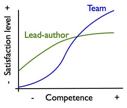
If you read last post you know I am experimenting with working in teams. I tend to think in graphs, so here is the conclusion I reach so far:

Teams.001

By “Satisfaction” I meant satisfaction of the leader or of the team, and involves quality of the paper, how much fun we had writing it, how innovative it is, etc*… By “Competence” I also meant competence of the lead author or of the team regarding the topic, stats, ideas… While for the lead author there is a lot on being good at integrating coauthors feed-back, for teams it also involves getting along really well. This graph is only a feeling, but I think that while teams can accomplish better results when they work hard, a single author is most likely to have moderate success even when the overall performance is low.

I think good teams need time to really get along. I also think working in the same space helps, but with email, tweeter, etc… may be is not that important anymore. I also think that 3-4 people is the key number to work in team, as is not realistic in my opinion to have more than 5 people fully involved without discussing badly.

Anyone with experiences to share?

*yes, ect… includes impact factor.

Are the tools we use shaping the way we collaborate?

This is the first of some thoughts about collaboration. I am quite convinced that working in teams enhance creativity, is more fun, and more productive, but is not always straightforward how to get the most out of our collaborations. Recently, I started wondering if the tools we use shape the way we collaborate. Let me put an example, the typical use of the track changes (in Word, OpenOffice, or whatever you want) predisposes you to have a leading author “accepting” or “rejecting” other people changes. On the other side, if you use a Git stile workflow, the system only show you where the changes are in the document, and (at least for me) kind of assumes you will accept those (if you don’t spot anything wrong). Don’t stop reading, this is not a typical “I hate Word” post and the next examples are all using a text processor.

What I am trying to say is that if you want a lead author supervising everything, you should use track changes, but when you aim for a more equal contribution, where all team members are expected to come to an agreement, track changes is against the flow of work. I don’t think is only a matter of how do you prefer to see the changes, but that it actually affects (unconsciously) people feelings and behaviours. For example, as a non-lead author, you don’t feel the project as yours as you should, and you are probably tempted to point out where the project needs to be enhanced, rather than enhancing it yourself. This feeling of “the lead-author will check if what I am editing reads ok” calls for sloppier edits. But in a team with no one accepting formally your changes, you are more likely to work until your changes read perfectly.

I’ve been experimenting with this in a couple of places. We agreed with Rachael on not using track changes for our F1000 evaluations. Those are short pieces and usually only need a couple of revision rounds among us (now in .txt format, way lighter than a word file*). It works perfectly. I am also co-leading a paper where we tried not to use track changes for writing the discussion. It only half worked here. At the beginning we didn’t agree on the structure, so we re-write a lot each other versions, and that felt time-consuming. I recognize it is hard to let go the control upon something you wrote. However at the end I am positive as the discussion is now a real (good) mix of our ideas and stiles. I have to say that we were working on the same office, so that helps a lot to solve questions in real-time.

Where I am going? I don’t know, and I did a lengthier post than usual, so I’ll write about pro’s and con’s of teams vs. lead authors in a couple of days.

———-
* ok, here is my “I hate word” rant.

Dear Journal

As a reviewer you should be allowed to answer review request using the same journal slang. Here is my version adapted to Science:

“Thank you for offering me to review the manuscript [Insert title here]. Competition for my time allocated to review is becoming increasingly fierce; I currently receive close to 30 requests a year, but I am only able to review roughly 12. The topic is certainly in my area of expertise and the analysis is interesting, however it was given a lower priority ranking than others. Unfortunately, this means that I will not be able to review it in-depth. My decisions are made on the basis of current workload as well as interest and significance. Due to my time limitations, I must reject excellent, exciting, and potentially important papers every month. Thus, my inability to review this work should not be taken as a direct comment on its quality or importance.” *

This is clearly ironic, and highlights the pressure to find reviewers, but honestly, I feel sorry every single time I have to say no to a review request, and I always want to write back explaining why I can’t this time.

*The acceptance to review version can also be quite interesting.